Transformer Theory for Computer Vision

Introduction to Transformers

Transformers have revolutionized the field of deep learning since their introduction in the 2017 paper “Attention is All You Need” by Vaswani et al. Originally designed for natural language processing (NLP) tasks, transformers have since been adapted for computer vision applications with remarkable success. This section covers the foundational theory of transformers, with a focus on their application to computer vision tasks.

The transformer architecture represents a paradigm shift in deep learning, moving away from recurrent and convolutional architectures toward a design that relies entirely on attention mechanisms. This shift has enabled models to capture long-range dependencies more effectively and process data in parallel, leading to significant improvements in performance across various tasks.

The Attention Mechanism: The Core of Transformers

Self-Attention Explained

The key innovation in transformer models is the self-attention mechanism, which allows the model to weigh the importance of different parts of the input data. Unlike recurrent neural networks (RNNs) or convolutional neural networks (CNNs), which process data sequentially or locally, self-attention can directly model relationships between all positions in a sequence.

In the context of transformers, attention mechanisms serve to weigh the influence of different input tokens when producing an output. The self-attention mechanism computes a weighted sum of all tokens in a sequence, where the weights are determined by the compatibility between the query and key representations of the tokens.

To understand self-attention more intuitively, consider how humans read text. When we encounter a pronoun like “it,” we naturally look back at the text to determine what “it” refers to. Similarly, self-attention allows a model to “look” at all other positions in the input to better understand the context of each position. This ability to consider the entire context simultaneously is what gives transformers their power.

Figure 2: Self-Attention Mechanism showing how Query (Q), Key (K), and Value (V) vectors are derived from input embeddings and interact to produce weighted outputs. The Query represents 'what we're looking for,' the Key represents 'what we have,' and the Value represents 'what we'll return if there's a match.'

Scaled Dot-Product Attention

The transformer implements a scaled dot-product attention, which follows these steps:

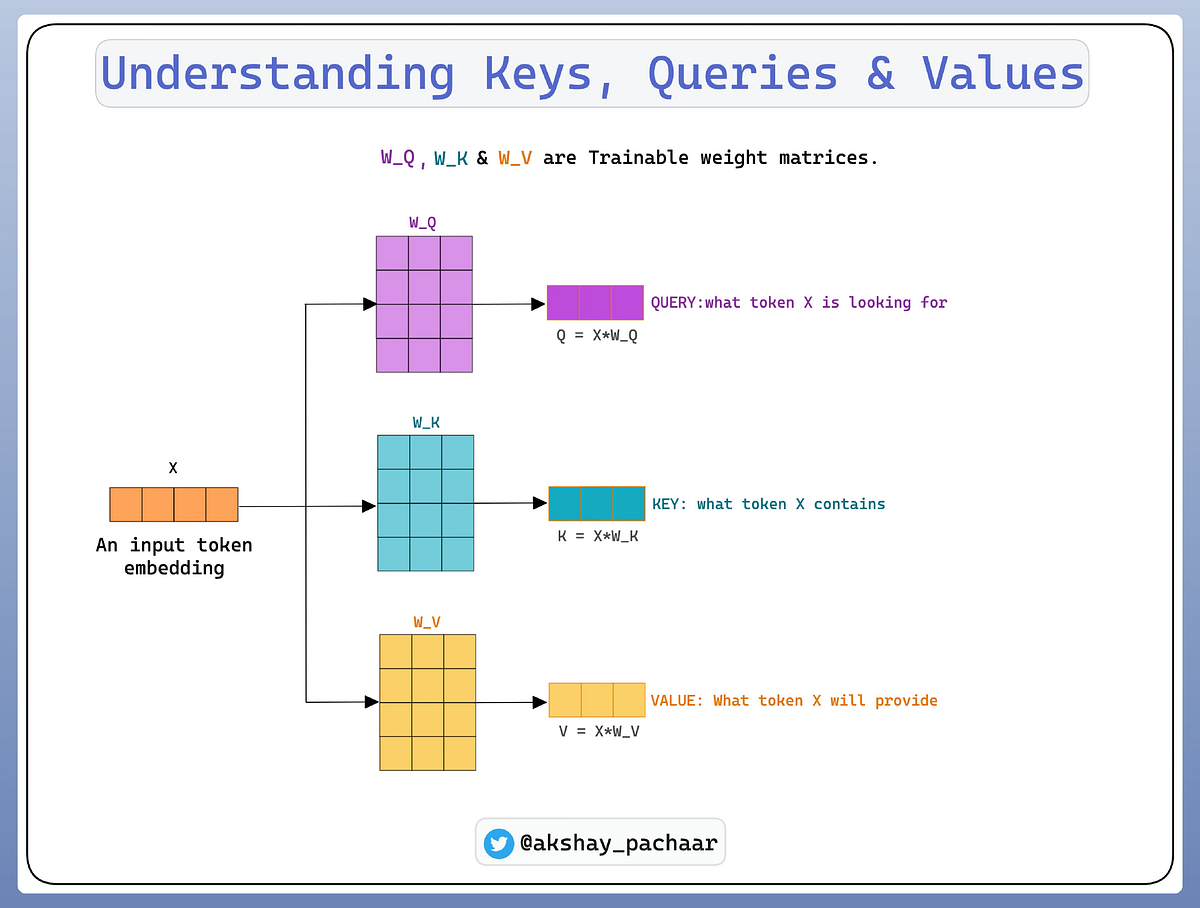
For each position in the input sequence, create three vectors: Query (Q), Key (K), and Value (V)
Calculate attention scores by taking the dot product of the query with all keys
Scale the scores by dividing by the square root of the dimension of the key vectors
Apply a softmax function to obtain the weights
Multiply each value vector by its corresponding weight and sum them to produce the output

Mathematically, this is represented as:

\[\text{Attention}(Q, K, V) = \text{softmax}\left(\frac{QK^T}{\sqrt{d_k}}\right) \cdot V\]

Where:

\(Q, K, V\) are matrices containing the queries, keys, and values
\(d_k\) is the dimension of the key vectors
The scaling factor √d_k prevents the softmax function from having extremely small gradients

The scaling factor is crucial because as the dimension of the key vectors increases, the dot products can grow large in magnitude, pushing the softmax function into regions with extremely small gradients. This scaling helps maintain stable gradients during training, allowing the model to learn more effectively.

Multi-Head Attention

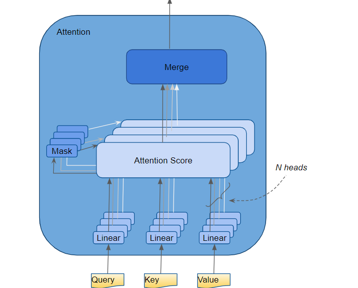
To enhance the model’s ability to focus on different positions and representation subspaces, transformers use multi-head attention. This involves:

Linearly projecting the queries, keys, and values multiple times with different learned projections
Performing the attention function in parallel on each projection
Concatenating the results and projecting again

This allows the model to jointly attend to information from different representation subspaces at different positions, providing a richer understanding of the input data.

Multi-head attention can be thought of as having multiple “representation subspaces” or “attention heads,” each focusing on different aspects of the input. For example, in language processing, one head might focus on syntactic relationships, while another might focus on semantic relationships. By combining these different perspectives, the model gains a more comprehensive understanding of the data.

The mathematical formulation for multi-head attention is:

\[\text{MultiHead}(Q, K, V) = \text{Concat}(\text{head}_1, \text{head}_2, ..., \text{head}_h) \cdot W^O\]

Where:

\[\text{head}_i = \text{Attention}(Q \cdot W_i^Q, K \cdot W_i^K, V \cdot W_i^V)\]

And \(W_i^Q\), \(W_i^K\), \(W_i^V\), and \(W^O\) are learned parameter matrices.

Transformer Architecture

Overall Structure

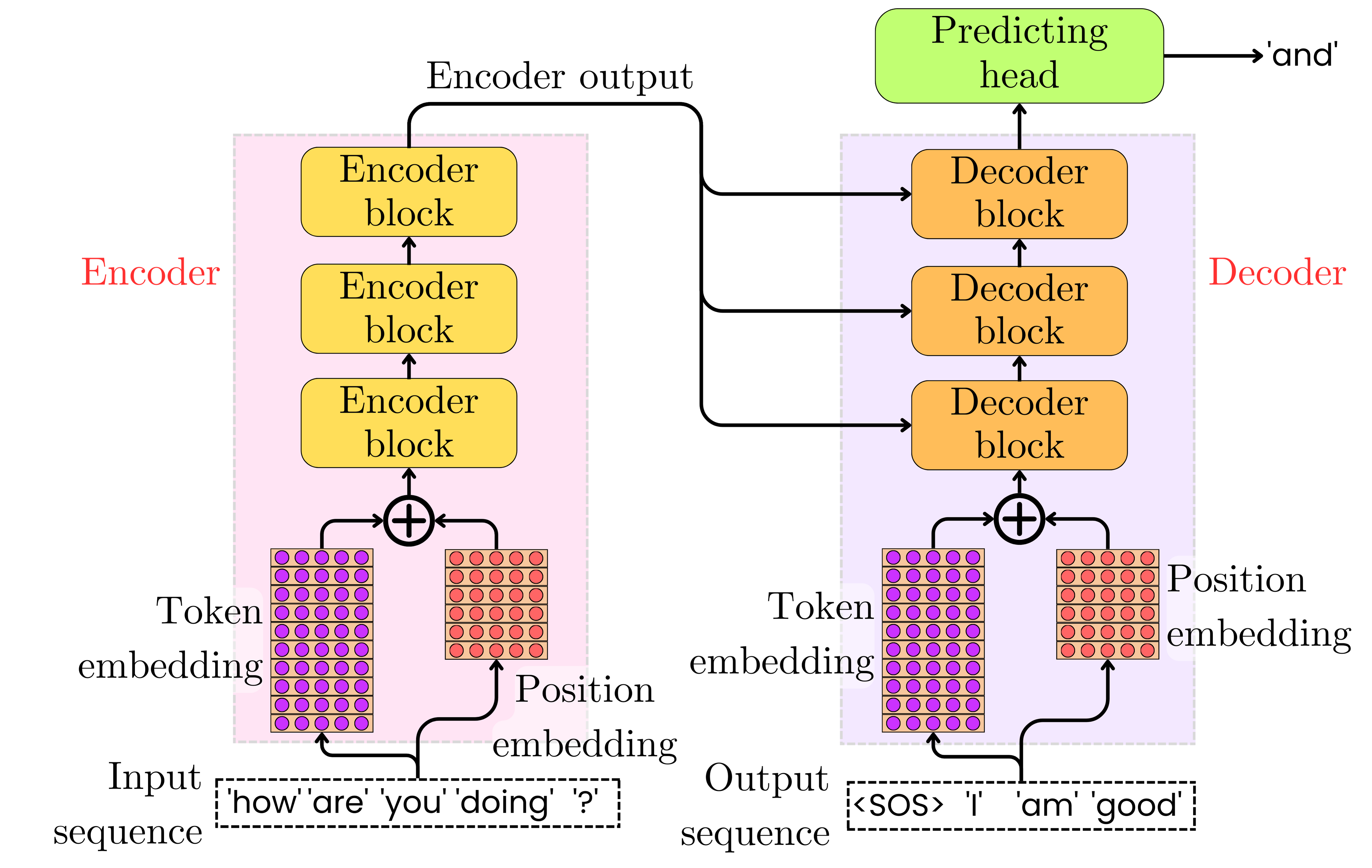
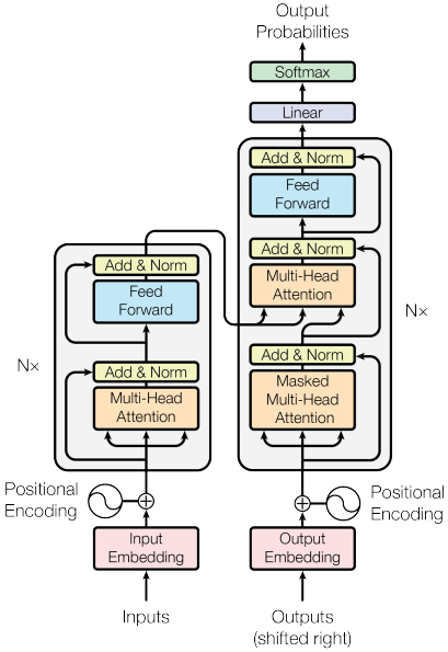
A transformer consists of an encoder and a decoder, each composed of multiple identical layers. Each layer has two main components:

A multi-head self-attention mechanism
A position-wise fully connected feed-forward network

Additionally, each sublayer employs residual connections and layer normalization to facilitate training.

The transformer architecture is designed to be highly parallelizable, allowing for efficient training on modern hardware. Unlike RNNs, which process tokens sequentially, transformers can process all tokens in parallel, significantly reducing training time for large datasets.

The Feed-Forward Network

The feed-forward network is a critical component in both the encoder and decoder layers of the transformer. It processes each position independently and identically, applying the same transformation to each representation.

This component serves several important purposes:

It adds non-linearity to the model, allowing it to learn more complex patterns
It transforms the attention-weighted representations into a form suitable for the next layer
It increases the model’s capacity by introducing additional parameters

The dimensionality of the inner layer (between \(W_1\) and \(W_2\)) is typically larger than the model dimension, often by a factor of 4. This expansion and subsequent projection allow the network to capture more complex relationships before compressing the information back to the model dimension.

The Encoder

The encoder processes the input sequence and generates representations that capture the contextual relationships within the data. It transforms the input tokens into a continuous representation that encodes the full context of the sequence.

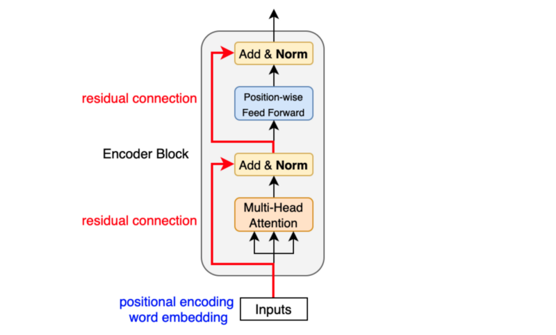
Encoder Architecture — Figure 3: Transformer Encoder Block showing the multi-head attention mechanism, position-wise feed-forward network, and the residual connections with layer normalization.

Each encoder layer consists of two main sub-layers:

Multi-Head Self-Attention Layer: This mechanism allows each position to attend to all positions in the previous layer. The self-attention operation enables the encoder to weigh the importance of different tokens when creating the representation for each position. For example, when encoding the word “bank” in the sentence “I went to the bank to deposit money,” the self-attention mechanism would give higher weight to words like “deposit” and “money” to understand that “bank” refers to a financial institution rather than a riverbank.
Position-wise Feed-Forward Network: After the attention mechanism, each position passes independently through an identical feed-forward network. This network consists of two linear transformations with a ReLU activation in between:
\[\text{FFN}(x) = \max(0, xW_1 + b_1)W_2 + b_2\]
This component adds non-linearity to the model and allows it to transform the attention-weighted representations further.
Layer Normalization and Residual Connections: Each sub-layer is wrapped with a residual connection followed by layer normalization. The residual connections (shown in red in the diagram) help with gradient flow during training, while layer normalization stabilizes the learning process by normalizing the inputs across features.

The encoder’s self-attention mechanism allows it to create contextual representations of each input token, taking into account the entire input sequence. This is particularly valuable for tasks where understanding the relationships between different parts of the input is crucial. Multiple encoder layers are typically stacked on top of each other, with each layer refining the representations from the previous layer.

The Decoder

The decoder generates the output sequence one element at a time in an autoregressive manner. This component is responsible for transforming the encoder’s representations into the final output sequence, such as translated text in a machine translation task.

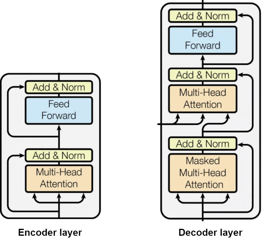
Decoder Architecture — Figure 4: Transformer Decoder Block showing the masked self-attention, encoder-decoder attention, and feed-forward layers with their respective normalization. Note the visual consistency with the encoder block architecture.

Each decoder layer includes three main sub-layers:

Masked Multi-Head Self-Attention: This first attention mechanism operates on the decoder’s own outputs from the previous layer. The “masked” aspect is crucial - it prevents positions from attending to subsequent positions by applying a mask to the attention scores before the softmax operation. This masking ensures that predictions for position i can only depend on known outputs at positions less than i, preserving the autoregressive property necessary for generation tasks.
Multi-Head Encoder-Decoder Attention: This second attention layer is what connects the decoder to the encoder. Here, queries come from the decoder’s previous layer, while keys and values come from the encoder’s output. This allows each position in the decoder to attend to all positions in the input sequence, creating a direct information pathway from input to output. This cross-attention mechanism is what allows the model to focus on relevant parts of the source sequence when generating each target token.
Position-wise Feed-Forward Network: Identical to the one in the encoder, this fully connected feed-forward network applies the same transformation to each position independently.

Each of these sub-layers is followed by a residual connection and layer normalization, similar to the encoder. This combination helps maintain stable gradients during training and allows for deeper networks.

Decoder Operation in Detail

The decoder operates sequentially during inference, generating one token at a time:

The decoder starts with a special start-of-sequence token and positional encoding.
For each new token position:

The masked self-attention ensures the decoder only considers previously generated tokens.
The encoder-decoder attention allows the decoder to focus on relevant parts of the input sequence.
The feed-forward network and final linear layer transform the representations into output probabilities.
The token with the highest probability is selected (or sampling is used) and added to the sequence.
This process repeats until an end-of-sequence token is generated or a maximum length is reached.

The decoder’s masked self-attention is what enables autoregressive generation. By masking future positions during training, the model learns to predict the next token based only on previously generated tokens, which is essential for tasks like machine translation or text generation.

The encoder-decoder attention mechanism serves as a dynamic, content-based alignment between input and output sequences. Unlike traditional sequence-to-sequence models with fixed attention mechanisms, this dynamic attention allows the model to adaptively focus on different parts of the input depending on what it’s currently generating, leading to more accurate and contextually appropriate outputs.

Positional Encoding

Since transformers do not inherently process sequential information, positional encodings are added to the input embeddings to provide information about the relative or absolute position of tokens in the sequence. These encodings have the same dimension as the embeddings, allowing them to be summed.

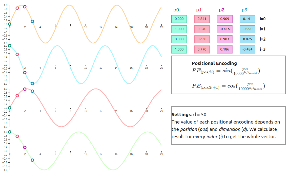
The original transformer paper used sine and cosine functions of different frequencies to create these positional encodings:

\[PE(pos, 2i) = \sin(pos / 10000^{(2i/d_{\text{model}})}) \\ PE(pos, 2i+1) = \cos(pos / 10000^{(2i/d_{\text{model}})})\]

Where:

\(pos\) is the position
\(i\) is the dimension
\(d_{\text{model}}\) is the embedding dimension

These encodings have the useful property that for any fixed offset k, PE(pos+k) can be represented as a linear function of PE(pos), which helps the model learn relative positions more easily.

Positional encodings are crucial for transformers because, unlike RNNs or CNNs, the self-attention operation is permutation-invariant—it doesn’t inherently know the order of the input sequence. By adding positional information to the token embeddings, the model can distinguish between tokens at different positions and understand the sequential nature of the data.

From NLP to Computer Vision: Vision Transformers (ViT)

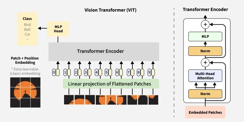
Adapting Transformers for Images

Vision Transformers (ViT) adapt the transformer architecture for image processing tasks. The key insight is to treat an image as a sequence of patches, similar to how words are treated in NLP applications.

The process involves:

Splitting the image into fixed-size patches (typically 16×16 pixels)
Flattening each patch into a vector
Linearly projecting these vectors to obtain patch embeddings
Adding position embeddings to retain spatial information
Processing the resulting sequence through a standard transformer encoder

Vision Transformer Architecture — Figure 6: Vision Transformer (ViT) architecture showing how an image is divided into patches, which are then linearly embedded, combined with position embeddings, and processed through a transformer encoder.

This approach differs significantly from traditional CNN architectures, which use convolutional layers to process images hierarchically. The self-attention mechanism in transformers allows ViT to capture global dependencies directly, without the need for multiple layers of convolution and pooling to increase the receptive field.

The ViT Architecture in Detail

The Vision Transformer architecture consists of the following components:

Patch Embedding: The input image is divided into non-overlapping patches, which are then flattened and linearly projected to create patch embeddings. For example, a 224×224 pixel image divided into 16×16 patches would result in 196 patches (14×14), each represented as a vector.
Class Token: A learnable embedding (CLS token) is prepended to the sequence of patch embeddings. The final representation of this token is used for image classification tasks.
Position Embedding: Since transformers have no inherent understanding of spatial relationships, position embeddings are added to the patch embeddings to provide information about the spatial arrangement of patches.
Transformer Encoder: The resulting sequence of embeddings is processed through multiple layers of a standard transformer encoder, which consists of multi-head self-attention and MLP blocks, with layer normalization and residual connections.
MLP Head: For classification tasks, final representation of the CLS token is passed through an MLP head to produce class predictions.

class VisionTransformer(nn.Module):
    def __init__(self, img_size=224, patch_size=16, in_chans=3, num_classes=1000,
                 embed_dim=768, depth=12, num_heads=12, mlp_ratio=4., qkv_bias=True):
        super().__init__()
        self.patch_embed = PatchEmbed(img_size, patch_size, in_chans, embed_dim)
        num_patches = self.patch_embed.num_patches

        # Create class token and position embeddings
        self.cls_token = nn.Parameter(torch.zeros(1, 1, embed_dim))
        self.pos_embed = nn.Parameter(torch.zeros(1, num_patches + 1, embed_dim))

        # Transformer encoder
        self.blocks = nn.ModuleList([
            Block(embed_dim, num_heads, mlp_ratio, qkv_bias)
            for _ in range(depth)
        ])

        # MLP head for classification
        self.norm = nn.LayerNorm(embed_dim)
        self.head = nn.Linear(embed_dim, num_classes)

Key Innovations in Vision Transformers

Vision Transformers introduced several key innovations that enabled transformers to be effectively applied to computer vision tasks:

Patch-based Image Representation: By treating image patches as tokens, ViT adapts the transformer architecture to process visual data without significantly modifying the original transformer design.
Pre-training on Large Datasets: ViT demonstrated that with sufficient pre-training data (e.g., JFT-300M), transformers can outperform CNNs on image classification tasks without incorporating image-specific inductive biases.
Transfer Learning: Pre-trained ViT models can be effectively fine-tuned on smaller datasets, making them practical for a wide range of computer vision applications.

Despite their success, early Vision Transformers had some limitations:

They required large amounts of training data to achieve competitive performance compared to CNNs.
The computational complexity of self-attention (quadratic in the number of patches) limited their application to high-resolution images.
They lacked some of the inductive biases that make CNNs effective for vision tasks, such as translation equivariance and locality.

These limitations have been addressed in subsequent transformer-based vision models.

Advancements Beyond Basic ViT

Since the introduction of the original Vision Transformer, numerous advancements have been made to address its limitations and improve its performance:

Hierarchical Transformers: Models like Swin Transformer introduce a hierarchical structure with local attention windows, making them more efficient and effective for high-resolution images and dense prediction tasks.
Hybrid Architectures: Combining convolutional layers with transformer blocks to leverage the strengths of both approaches, as seen in models like ConViT and CvT.
Efficient Attention Mechanisms: Developing more efficient attention variants to reduce the computational complexity of self-attention, such as linear attention and sparse attention.
Data-efficient Training: Techniques like DeiT (Data-efficient image Transformers) show that with appropriate training strategies, ViTs can be trained effectively on smaller datasets without extensive pre-training.

Vision Transformers have revolutionized computer vision by demonstrating that the transformer architecture, originally designed for NLP tasks, can be highly effective for visual tasks as well. This cross-domain success has led to a convergence of techniques across modalities and inspired a new generation of models that leverage the strengths of both transformers and CNNs.

The rapid advancement of transformer-based vision models continues to push the state-of-the-art in computer vision, with applications ranging from image classification and object detection to segmentation, video understanding, and multimodal learning.

Advanced Transformer Variants for Computer Vision

Swin Transformer

The Swin (Shifted Window) Transformer introduces hierarchical feature maps and shifted windowing to improve efficiency and performance. Key innovations include:

Hierarchical Feature Maps: Merging patches progressively to create a hierarchical representation. This is similar to the feature pyramid in CNNs and allows the model to capture multi-scale features efficiently. At each stage, neighboring patches are merged, reducing the sequence length while increasing the feature dimension.
Window-based Self-Attention: Computing self-attention within local windows to reduce computational complexity. Instead of performing self-attention across the entire image, which scales quadratically with image size, Swin Transformer restricts attention to local windows. This reduces the computational complexity to linear with respect to image size.
Shifted Window Partitioning: Alternating between regular and shifted window partitioning to enable cross-window connections. In one layer, the image is divided into non-overlapping windows; in the next layer, the window partitioning is shifted, creating connections between previously separate windows. This allows information to flow across the entire image while maintaining computational efficiency.

The Swin Transformer’s hierarchical design and efficient attention mechanism make it particularly well-suited for dense prediction tasks like object detection and semantic segmentation, where multi-scale feature representations are important.

DeiT (Data-efficient image Transformers)

DeiT demonstrates that Vision Transformers can be trained effectively on smaller datasets through:

Distillation Token: A specific token that learns from a teacher model (typically a CNN). In addition to the class token, DeiT introduces a distillation token that is supervised by the output of a pre-trained CNN. This allows the model to leverage the inductive biases of CNNs without explicitly incorporating them into the architecture.
Strong Data Augmentation: Techniques like RandAugment and CutMix to increase data diversity. These augmentations create a more varied training set, helping the model generalize better from limited data. RandAugment applies a series of random transformations to each image, while CutMix combines patches from different images along with their labels.
Regularization: Methods to prevent overfitting on smaller datasets. DeiT employs techniques like stochastic depth (randomly dropping layers during training) and weight decay to improve generalization.

DeiT’s approach shows that with appropriate training techniques, transformers can achieve competitive performance even without the massive pre-training datasets used in the original ViT paper.

MobileViT

MobileViT combines the strengths of CNNs and transformers for mobile applications:

Local Processing: Using convolutions for local feature extraction. MobileViT starts with convolutional layers to efficiently capture local patterns and reduce the spatial dimensions of the input.
Global Understanding: Applying transformers for global context modeling. After the initial convolutional processing, transformer blocks are used to capture long-range dependencies and global context.
Lightweight Design: Optimized architecture for mobile devices with limited computational resources. MobileViT uses depth-wise separable convolutions and efficient transformer implementations to reduce the number of parameters and computational cost.

This hybrid approach leverages the strengths of both architectures—the efficiency and local processing capabilities of CNNs, and the global modeling capabilities of transformers—making it well-suited for deployment on resource-constrained devices.

Attention Mechanisms Beyond Transformers

Non-local Neural Networks

Non-local neural networks capture long-range dependencies by computing the response at a position as a weighted sum of features at all positions. This is conceptually similar to self-attention but was developed independently.

The non-local operation can be expressed as:

\[y_i = \frac{1}{C(x)} \sum_j f(x_i, x_j) g(x_j)\]

Where:

\(x_i\) is the input feature at position i
\(y_i\) is the output feature at position i
\(f(x_i, x_j)\) computes a scalar representing the relationship between positions i and j
\(g(x_j)\) computes a representation of the input at position j
\(C(x)\) is a normalization factor

This operation allows the model to consider all positions when computing the output for each position, capturing global context. Non-local neural networks have been successfully applied to video understanding, where capturing temporal dependencies is crucial.

Squeeze-and-Excitation Networks

Squeeze-and-Excitation networks adaptively recalibrate channel-wise feature responses by explicitly modeling interdependencies between channels, providing a form of attention over feature channels.

The SE block consists of two operations:

Squeeze: Global average pooling to extract channel-wise statistics
Excitation: A gating mechanism with two fully connected layers and a sigmoid activation to generate channel-wise attention weights

Mathematically, for input feature map U:

\[z = F_{\text{sq}}(U) = \text{GlobalAveragePooling}(U) \\ s = F_{\text{ex}}(z) = \sigma(W_2 \cdot \text{ReLU}(W_1 \cdot z)) \\ \hat{U} = s \cdot U\]

Where:

\(z\) is the squeezed representation
\(s\) is the channel-wise attention weights
\(\hat{U}\) is the recalibrated feature map
\(W_1\) and \(W_2\) are learnable parameters

SE networks improve performance by allowing the model to emphasize informative features and suppress less useful ones, with minimal additional computational cost.

CBAM (Convolutional Block Attention Module)

CBAM combines channel and spatial attention to enhance the representational power of CNNs, focusing on “what” and “where” to attend in the feature maps.

CBAM consists of two sequential sub-modules:

Channel Attention Module: Similar to SE networks, it focuses on “what” is meaningful in the input features
Spatial Attention Module: Focuses on “where” to attend by generating a spatial attention map

The process can be summarized as:

\[F' = M_c(F) \otimes F \\ F'' = M_s(F') \otimes F'\]

Where:

\(F\) is the input feature map
\(M_c\) is the channel attention map
\(M_s\) is the spatial attention map
⊗ represents element-wise multiplication

CBAM provides a complementary attention mechanism to the self-attention used in transformers, focusing on different aspects of the input data.

Practical Applications of Vision Transformers

Vision Transformers have demonstrated impressive performance across a wide range of computer vision tasks:

Image Classification: ViTs have achieved state-of-the-art results on benchmark datasets like ImageNet, particularly when pre-trained on large datasets.
Object Detection: Models like DETR (DEtection TRansformer) use transformers to directly predict object bounding boxes and classes, eliminating the need for hand-designed components like anchor boxes and non-maximum suppression.
Semantic Segmentation: Transformer-based models can generate pixel-level predictions for scene understanding, benefiting from their ability to capture long-range dependencies.
Image Generation: Models like DALL-E and Stable Diffusion use transformer architectures to generate high-quality images from text descriptions, showcasing the versatility of transformers beyond discriminative tasks.
Video Understanding: Transformers can process spatio-temporal data for tasks like action recognition and video captioning, leveraging their ability to model relationships across both space and time.
Multi-modal Learning: Transformers excel at integrating information from different modalities, such as text and images, enabling applications like visual question answering and image captioning.

Glossary of Key Terms

Attention: A mechanism that allows models to focus on relevant parts of the input when producing an output.
Self-Attention: A specific form of attention where the query, key, and value all come from the same source.
Query, Key, Value (Q, K, V): The three components used in attention mechanisms. The query represents what we’re looking for, the key represents what we have, and the value represents what we’ll return if there’s a match.
Multi-Head Attention: Running multiple attention operations in parallel and concatenating the results.
Encoder: The part of the transformer that processes the input sequence and generates representations.
Decoder: The part of the transformer that generates the output sequence based on the encoder’s representations.
Positional Encoding: Information added to token embeddings to provide the model with information about the position of each token.
Vision Transformer (ViT): An adaptation of the transformer architecture for image processing tasks.
Patch Embedding: The process of dividing an image into patches and projecting them into a high-dimensional space.
Class Token: A special token added to the sequence of patch embeddings in ViT, used for classification tasks.
Inductive Bias: The set of assumptions that a model makes to generalize from training data to unseen data.

Conclusion

Transformers have fundamentally changed how we approach computer vision tasks. By leveraging self-attention mechanisms, they can capture global dependencies and relationships within images more effectively than traditional architectures. Vision Transformers and their variants have demonstrated state-of-the-art performance across various computer vision tasks, from image classification to object detection and segmentation.

The success of transformers in computer vision highlights the value of cross-pollination between different domains of deep learning. As research continues, we can expect further innovations that combine the strengths of transformers with other architectural paradigms, leading to more efficient and effective models for computer vision applications.

References

Vaswani, A., Shazeer, N., Parmar, N., Uszkoreit, J., Jones, L., Gomez, A. N., … & Polosukhin, I. (2017). Attention is all you need. In Advances in neural information processing systems.
Dosovitskiy, A., Beyer, L., Kolesnikov, A., Weissenborn, D., Zhai, X., Unterthiner, T., … & Houlsby, N. (2021). An image is worth 16x16 words: Transformers for image recognition at scale. In International Conference on Learning Representations.
Liu, Z., Lin, Y., Cao, Y., Hu, H., Wei, Y., Zhang, Z., … & Guo, B. (2021). Swin transformer: Hierarchical vision transformer using shifted windows. In Proceedings of the IEEE/CVF International Conference on Computer Vision.
Touvron, H., Cord, M., Douze, M., Massa, F., Sablayrolles, A., & Jégou, H. (2021). Training data-efficient image transformers & distillation through attention. In International Conference on Machine Learning.
Mehta, S., & Rastegari, M. (2021). MobileViT: Light-weight, General-purpose, and Mobile-friendly Vision Transformer. arXiv preprint arXiv:2110.02178.
Wang, X., Girshick, R., Gupta, A., & He, K. (2018). Non-local neural networks. In Proceedings of the IEEE conference on computer vision and pattern recognition.
Hu, J., Shen, L., & Sun, G. (2018). Squeeze-and-excitation networks. In Proceedings of the IEEE conference on computer vision and pattern recognition.
Woo, S., Park, J., Lee, J. Y., & Kweon, I. S. (2018). Cbam: Convolutional block attention module. In Proceedings of the European conference on computer vision.
Alammar, J. (2018). The Illustrated Transformer. https://jalammar.github.io/illustrated-transformer/
Machine Learning Mastery. (2023). The Transformer Attention Mechanism. https://www.machinelearningmastery.com/the-transformer-attention-mechanism/